

Synchronous vs. Asynchronous Communication
The main distinctive feature of a serial communication system is that data is handled in series, i. e. bit by bit. The simplest serial communication device is the shift register. Consider the example in Fig. 3.1, where two shift registers are connected in such a way that the content of the first, called the transmitter, is transferred to the second, called the receiver.
Note that, in this case, the shift clock CLK, and the control signals SH/LD\ and RSTR must be generated at the transmitter level, at precise moments of time (see Fig. 3.2.) and transmitted along with data on the communication line. Such a communication system, where the transmission clock is sent to the communication line, is called synchronous communication.
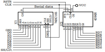
Fig. 3.1. Example of synchronous serial communication circuit
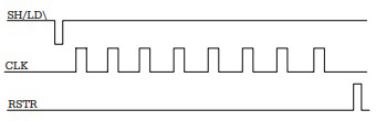
Fig. 3.2. Waveforms of the control signals for the circuit presented in Fig. 3.1
The problem becomes more complicated when it is not possible to send the serial clock over the communication line. In this situation, the receiver must generate its own clock, RxCLK, to shift data into the Rx shift register.
This type of serial communication, where the serial clock is not transmitted on the communication line, is called asynchronous communication. The generic block diagram of an asynchronous communication system is shown in Fig. 3.3.
To make this possible, the first requirement is that the transmitter and the receiver clock have exactly the same frequency. A limited number of possible frequencies have been standardized for asynchronous communication. These are: 110, 300, 600, 1200, 2400, 4800, 9600, 19 200, 57 600, 115 200 Hz.
Since the frequency of the transmission clock is directly related to the communication speed, so that with each clock pulse a bit of information is transmitted, the communication speed is measured in bits per second or baud. The period of the transmission clock is called the bit time Tb.
The second requirement is to mark somehow the beginning of the transmission of a sequence of bits. For this purpose, a special synchronization bit, called the start bit, has been inserted. This has the polarity opposed to the idle line status and its duration equals one TxCLK period.
The moment when the transmission ends is known, because the number of bits in each packet is known. In most cases, data is sent in 8-bit packets. To make sure the communication line returns to its idle status after each data packet is transmitted, an additional stop bit is transmitted. This always has the status of the idle line. Figure 3.4. shows how the data line is sampled at the receiver.
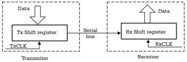
Fig. 3.3. Block diagram of an asynchronous communication system
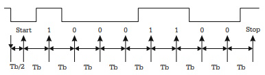
Fig. 3.4. Sampling data line in an asynchronous serial communication
The falling edge of the data line, corresponding to the start bit, starts the reception process.
The data line is sampled after half of the bit time interval to check for a valid start bit, and then at intervals equal to Tb. The values of the data line at these moments are shifted into the receiver data shift register Rx.
Error Detection in Asynchronous Communication
One serious problem when handling asynchronous serial communication is the vulnerability to electromagnetic interference. Several means have been provided to detect communication errors, and the status register of an asynchronous serial interface normally contains special status bits to indicate these errors.
If, for instance, when sampling the data line at the moment T0 + Tb/2 (refer to Fig. 3.4), a value of 1 is obtained, that means the falling edge detected at the moment T0 was not a valid start bit, but a spike due to electromagnetic noise. This type of error is called noise error.
Similarly, if the data line status at the moment T1 = T0 + Tb/2 + 9 × Tb is not HIGH, this means that the expected stop bit is invalid, indicating that the byte received is in error. This type of error is called framing error.
Obviously, these two control methods are insufficient to detect all possible errors. Another method to verify the integrity of data is parity control. For this purpose, a special bit, called the parity bit, is transmitted just before the stop bit. This is either the most significant bit of each byte, or an additional ninth bit attached to each byte.
The values of the parity bits are automatically set so that the total number of 1s contained in the byte, plus the parity bit, is always an ODD or EVEN number, at the user’s choice. Both the transmitter and receiver must calculate the parity according to the same rule (ODD or EVEN). Upon reception of each byte, the parity is calculated, and, if the parity does not match the rule, the error is reported.
Parity control still cannot detect all errors, but, at the hardware level, the methods described above are all that can be done for error detection. For better error detection, software techniques must be used. Basically, software detection of communication errors relies on the following principles:
• The communication is based on data packets, having a determined structure.
• Each data packet contains a special field reserved for a sophisticated checksum.
The transmitter computes the checksum for each packet and inserts it into the
reserved field of the packet.
• The receiver recalculates the checksum of the packet and compares it with the
value calculated by the transmitter and sent along with the packet. If the two
values don’t match the packet is rejected, and the transmitter is requested to
repeat the transmission of the packet.
This method is called Cyclic Redundancy Check Control (CRC). The algorithms used to compute the checksums are so complex that the probability that a packet with errors still has a correct checksum is extremely low.
The General Structure of the Asynchronous Serial Communication Interface
The general block diagram of an asynchronous serial interface is presented in Fig. 3.5. This circuit is called a Universal Asynchronous Receiver Transmitter (UART). There are numerous stand-alone integrated circuits with this function, but most microcontrollers include a simplified version of UART, with the generic name Serial Communication Interface (SCI). This chapter contains details on the implementation of the SCI of HC11, AVR and 8051 microcontrollers. Even though there are differences in what concerns the names of the registers associated with the interface, or the names and particular functions of the control and status bits, the general structure of the interface is basically the same in all microcontrollers.
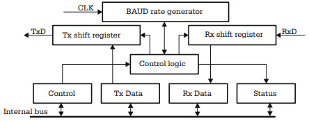
Fig. 3.5. General block diagram of the asynchronous serial communication interface
About Microcontrollers in Practice

The book is structured into three sections. Chapters 1-8 aim to create a detailed overview of microcontrollers, by presenting their subsystems starting from a general functional block diagram, valid for most microcontrollers on the market. In each case, we describe the distinctive features of that specific subsystem for HC11, 8051 and AVR. This whole section has a more theoretical approach, but, even here, many practical examples are presented, mainly regarding the initializations required by each subsystem, or the particular use of the associated interrupts. The purpose of this section is to create a perspective that views the microcontroller as a set of resources, easy to identify and use.
Chapters 9-16 contain eight complete projects, described from the initial idea, to the printed circuit board and detailed software implementation. Here too, we permanently focus on the similarities between the microcontrollers discussed, from the hardware and software perspectives.
All chapters contain exercises, suggesting modifications or improvements of the examples in the book. Most exercises have solutions in the book; for the others the solutions can be found on the accompanying CD.
Finally, the appendices contain additional information intended to help the reader to fully understand all the aspects of the projects described in the previous sections. We chose to present these details separately in these appendices, in order to avoid fragmentation of the flow of the main text.
Stressing common characteristics and real applications of the most used microcontrollers, this practical guide provides readers with hands-on knowledge of how to implement three families of microcontrollers (HC11, AVR, and 8051). Unlike the rest of the ocean of literature on individual chips, Microcontrollers in Practice supplies side-by-side comparisons and an overview that treats the systems as resources available for implementation. Packed with hundreds of practical examples and exercises to foster mastery of concepts and details, the guide also includes several extended projects. By treating the less expensive 8-bit and RISC microcontrollers, this information-dense manual equips students and home-experimenters with the know-how to put these devices into operation. Click here to learn more.

More Computer Architecture Articles:
• The Many Processes of Silicon Wafer Manufacturing
• Monolithic Kernel vs Microkernel vs Hybrid Kernel
• Fundamental Digital Logic Gates
• Binary Floating-Point Numbers
• Introduction to Microprocessor Programming
• Basic Electronics for Computer Architecture
• Electronic Circuits Basics
• The Microcontroller Interrupt System
• Multicore Programming
• Using the Microcontroller Timers